Moore’s Law Isn’t Dead: It’s Wrong - Long Live Wright’s Law

Yes, the most famous technology forecast of all time—Gordon Moore’s prediction that the number of transistors on a chip would double every two years—confuses why and how technology costs decline. It focuses on the wrong variable: time.

When he wrote “every two years” in forecasting the doubling of transistor density and consequent halving of computation costs,[1] Moore implicitly assumed that consumer demand would increase in tandem with production. If transistor demand had faltered, Moore’s Law would have failed: reducing the marginal cost of a chip would have done nothing but shrink the market. As a result, companies would not have invested in the research or production capacity to drive costs down. Moore’s Law was only a “law” because demand scaled enough to justify the increased investment.

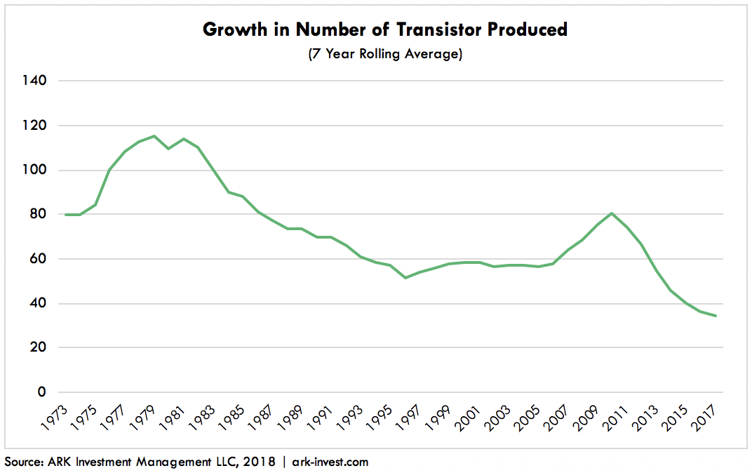
The assumption that costs would decline continually—tick tock, tick tock, the basis of Intel’s product innovation cycle,—has not withstood the test of time. Moore embedded in his Law an assumption that over time unit demand, and hence production volumes, would respond to continuous price declines. Empirically, and perhaps misunderstood by the marketplace, the growth in unit production of transistors has slowed dramatically over the course of this business cycle. As a consequence, and not surprisingly, the price decline for computation has begun to plateau. The public proclaims “the end of Moore’s Law”, not realizing that it has been flawed all along.

If Moore’s Law is flawed, what is the best way to forecast a technology cost decline? Instead of forecasting cost as a function of time, such a formula should incorporate the mechanic behind cost declines: production volume.

Another law, one that predates Gordon Moore’s pronouncement by nearly three decades, forecasts cost as a function of production: Wright’s Law. While studying production costs during the 1920s, Theodore Wright determined that for every cumulative doubling in the number of airplanes produced, manufacturers realized a consistent cost decline in percentage terms.[2] The cost to produce the 2,000^th plane was 15% less than that to produce the 1,000^th plane, and the cost to produce the 4,000^th plane, 15% less than that to produce the 2,000^th.

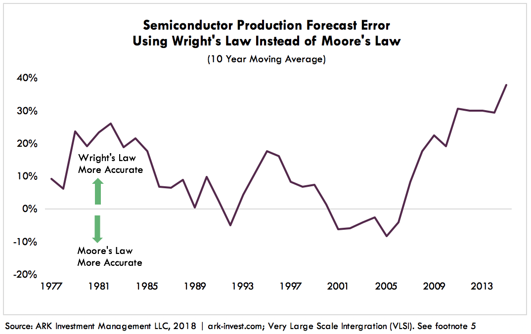
Wright’s Law extends to other industries. In recent years researchers at the Santa Fe Risk Institute concluded that it can forecast the cost decline associated with any technology.[3] In 2012 the researchers compared the forecast error rates between Moore’s Law and Wright’s Law across 62 technologies ranging from black and white TVs to photovoltaic cells, and from electric ovens to nuclear power. They concluded that Wright’s Law outperformed Moore’s Law consistently.  Even in his research on transistors, Gordon Moore would have been served better by applying Wright’s Law than creating Moore’s Law as a forecasting tool, as shown below.  Measured over the decade to 2015 (the latest data point available), a price forecast based on Wright’s Law was 40% more accurate than one based on Moore’s Law.[4] Measured across the entire data series Wright’s Law reduced the forecast error by 15% on average.

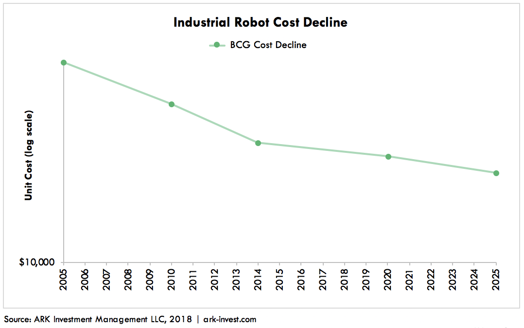
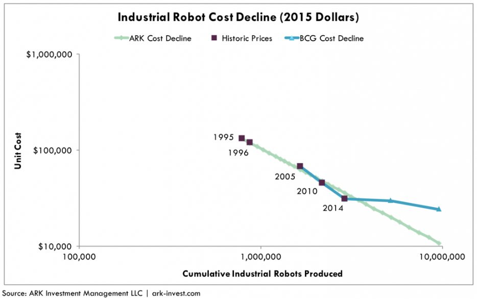
Although the superior methodology, Wright’s Law does face several challenges in projecting technology cost declines. First, it requires a long history of data. While forecasts based on Moore’s Law can be generated from the two most recent data points, Wright’s Law requires data on units produced not only during the last few years of the technology but throughout its history to determine the cost declines associated with every cumulative doubling of production. With just a few data points on the cost of industrial robots, for example, a researcher can forecast costs, as shown in the top chart below. With more history, however, that forecast looks too conservative, as shown in the second chart.

The second challenge associated with Wright’s Law involves anticipated demand. Moore’s Law suggests that as time passes, costs will fall. Wright’s Law requires an understanding of the price elasticity of demand, or how much demand will respond to future price declines. Having determined the “learning rate” at which costs will fall with every cumulative doubling of production, an analyst then has to determine the rate at which production will double cumulatively. For some technologies, demand can change discontinuously as costs and capabilities fall to tipping points that trigger mass market adoption.

Lithium-ion batteries offer a good case study. Based on the chart below, most analysts would conclude that lithium-ion batteries matured by 2005. After two decades of declining roughly 10% on average per year, lithium ion battery costs flattened out.

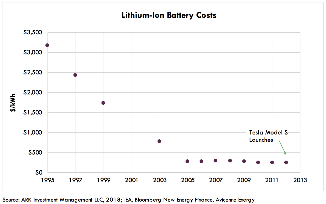
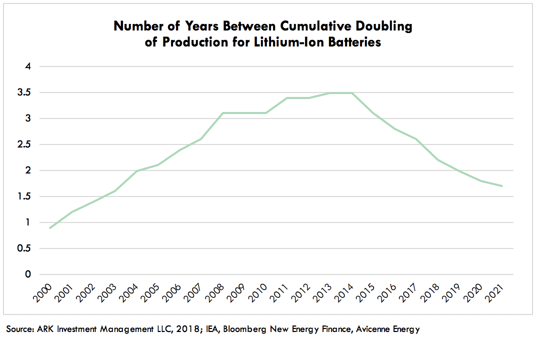
Unrecognized by most analysts, however, those 10% declines pushed the unit-cost of lithium-ion batteries across a critical threshold, enabling the production of electric vehicles at scale. One 200+ mile range electric vehicle has as much battery power as 5,000 iPhones, so if just 1% of auto sales were to convert from gas powered to electric, they would more than double the demand for batteries relative to those required for smartphones globally. Recognizing that batteries were about to hit this tipping point, analysts could have forecasted that the time required for the cumulative doubling of production would drop precipitously and that the decline in costs would reaccelerate, as shown in the two charts below.

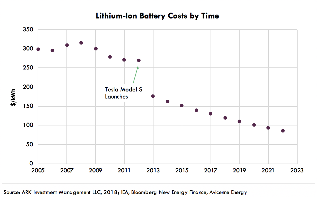
While a Moore’s Law style forecast deemed lithium-ion battery technology mature more than ten years ago, Wright’s Law correctly anticipated a reacceleration in cost declines and a resurgence in demand roughly five years ago. The decline in prices has opened up new segments of the auto market to lithium-ion batteries which, in turn, is pushing them toward an even larger market, utility-scale energy storage.

While the cost decline in batteries after the launch of Tesla’s Model S appears discontinuous when presented as a function of time, when recast using Wright’s Law –  costs presented as a function of unit production –  the cost drop appears neither discontinuous nor particularly surprising.

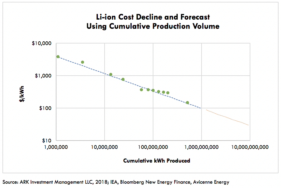
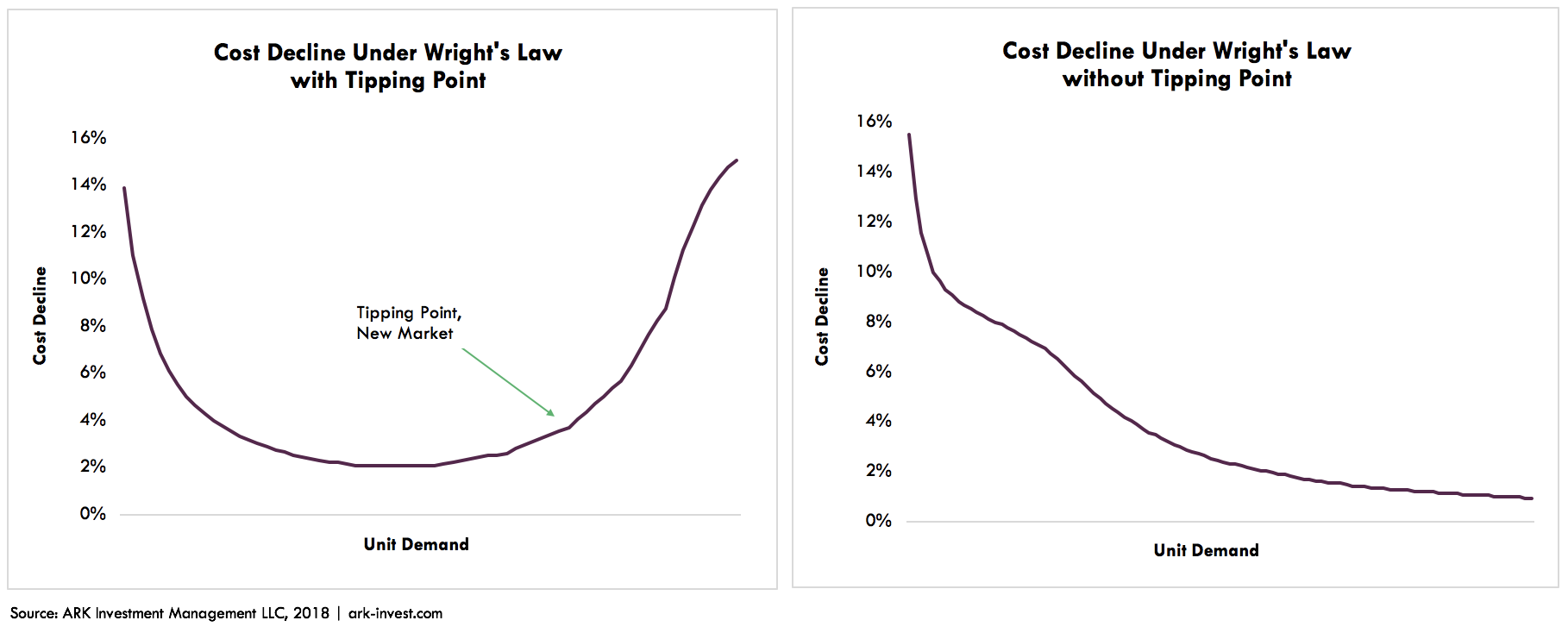
This insight from the EV market has broader applications. When a seemingly mature technology crosses critical demand thresholds, the decline in its cost trajectory will re-accelerate. As shown in the charts below, technologies crossing these thresholds drive accelerated cost curve declines that catch the market off guard, as has been the case with electric vehicles. At the same time, technologies that do not cross critical thresholds and do not unlock new markets stagnate, losing the cost curve declines that spur more innovation, disappointing expectations, also shown below.

From a technology investor’s perspective, when a trend is difficult to discern, requiring a painstaking reconstruction of history and a nuanced understanding of unit economics, Wright’s Law provides a powerful solution. Moore’s Law can provide a successful “short cut” for short-term forecasts in certain circumstances, but over longer time horizons it often leads forecasts astray. Seeking more durable answers and investment solutions, ARK takes the “long cut” associated with Wright’s Law.